|
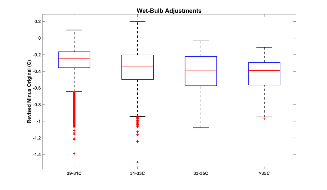
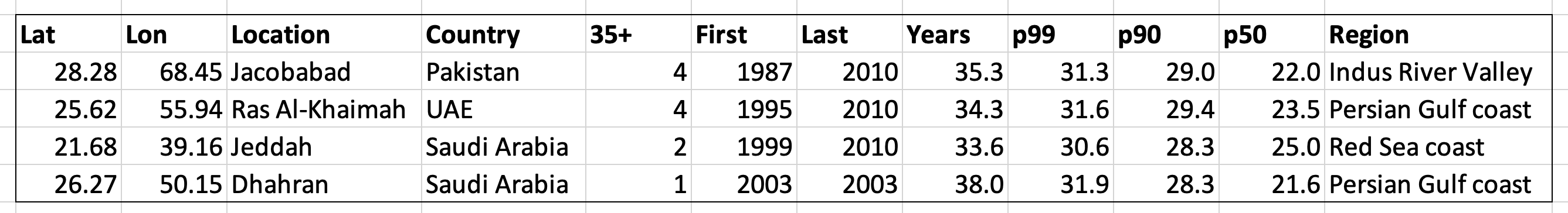
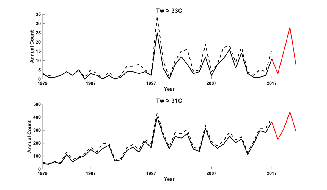
Wet-bulb temperature [Tw] is one of the fundamental metrics governing the workings of the atmosphere, as well as the impacts of weather and climate on humans and other endotherms. For these reasons, and because it captures combinations of temperature and humidity in a globally consistent, human-health-relevant way without relying on difficult-to-measure variables or calibrated indices, much of the foundational research on heat stress has used Tw as the metric of choice. While current understanding has moved beyond a one-to-one relationship between Tw values and physiological stresses, all comparable alternative metrics have similar interpretation caveats. Together with its large and growing base of supporting literature, this means that Tw will likely remain relevant for understanding humid heat stress for quite some time. In an operational sense, Tw's primary drawback is that most of the existing implementations calculate it through a computationally expensive iterative method. This effectively limits large-scale observational or modeling studies to researchers with access to ample processing power, and it hampers efforts to get a better handle on fine-scale spatiotemporal Tw patterns. The most commonly used algorithm is that developed by Davies-Jones (2008), implemented in Fortran 90 by Jonathan Buzan as part of the HumanIndexMod and later translated into MATLAB and Python versions by Bob Kopp and Xian-Xiang Li respectively. Second place in popularity probably goes to the Stull (2011) algorithm, despite its demonstrably larger biases for high heat-stress values, because it is at least an order of magnitude faster than the Davies-Jones codebase. The last year has seen a case of multiple discovery, as two groups have independently pursued approaches to increase the accuracy and efficiency of Tw calculations. [To be precise, this is referring to psychrometric adiabatic Tw, by far the most common Tw variety in climate science.] At the Bureau of Meteorology, Rob Warren and Cass Rogers have developed completely new code that efficiently computes Tw, while at the Jet Propulsion Lab Alex Goodman and I have revised the Buzan/Li implementation to incorporate Numba JIT optimizations. Through our correspondence with each other and with Jonathan Buzan, both groups have detected and removed several longstanding errors, as described further by Rob Warren in this document: 1. incorrect specification of the 'cold' regime 2. incorrect derivative in the main wet-bulb module 3. unnecessary approximations that a) assumed equivalency between specific humidity and mixing ratio and b) assumed relative humidity to be the ratio of actual and saturation mixing ratios (rather than actual and saturation vapor pressures) Code addressing (1) and (3) has been written by Rob Warren, while (2) was addressed several years ago by Qinqin Kong. The Goodman-Raymond Python implementation calculates 10^6 wet-bulb temperatures in about 0.3 seconds on a laptop, or about 50x faster than the Kopp MATLAB implementation, which it should be noted is no longer maintained. The Warren-Rogers implementation (also in Python) is similarly fast. Heritage code has its advantages, of course, but in this case we believe the community can significantly benefit from the adoption of faster and more accurate algorithms. The very success of the Kopp, X. Li, and possible other implementations is what motivates this effort to raise awareness of their need for correction. Code containing all three errors is almost certainly in wide circulation. What implications, then, do these revelations have for the interpretation of existing heat-stress literature? For the Kopp implementation (the X. Li Python implementation should behave very similarly), when calculating Tw with specific humidity as the input, the errors are rather small for realistic ranges of temperature and humidity (see document linked above for details). Errors 2 and 3 tend to create a negative bias, while error 1 slightly offsets them. With relative humidity as the input, the errors are larger, and error 3 in particular leads to a notable positive bias. Given the air-temperature and relative-humidity ranges associated with global extreme heat stress (see Figure S15 of Raymond et al. 2020), the total Tw error when using uncorrected code for these values is approximately -0.3 to -0.1 C when using specific humidity, or approximately +0.2 to +0.6 C when using relative humidity. A few calculations in very hot and dry climates (temperatures >=45C) have errors up to +1.0C. Re-evaluating the data underlying Raymond et al. 2020 illustrates and contextualizes these effects more concretely. Depending on the associated relative humidity, an original Tw value of 35.0C becomes 34.0-34.9C with the revisions, scattered around a median correction of -0.4C (Figure 1 below). Around Tw=30C, the correction is closer to -0.25C, and by 20C it is -0.1C. But even restricting our attention to the most extreme observed values, 11 of the 14 Tw>=35C occurrences noted in the paper remain above 35C after correction (Figure 2). The long-term global trends are negligibly affected, as might be expected, and in fact the addition of 2018-21 data arguably makes at least as big of an impact (Figure 3). This critical examination highlights the important point that while accurate code is no doubt important, the results of existing peer-reviewed heat-stress work should be robust to the biasing effects of the recently discovered errors, because a study that sensitive to small differences in Tw should not have been published in the first place. It is also worth emphasizing that this issue should not obscure the existence of other uncertainties attendant in heat-stress studies, many of them less easily quantifiable. For example, the details of the link between Tw and heat stress are subject to conflicting evidence (Baldwin et al. 2023) and to variations across environments and physiologies (Vecellio et al. 2022). Other metrics are difficult to calculate reliably across the globe or have their own idiosyncratic issues. The quantitative conclusions of past heat-stress studies thus might change slightly, but the qualitative ones do not, and certainly the aggregate findings stand up. For future studies using Tw, I would suggest one of several options: a) An off-the-shelf fresh codebase can be obtained: the Goodman-Raymond implementation is already available on Github, while the Warren-Rogers one (termed NEWT: Non-iterative Evaluation of Wet-bulb Temperature) is currently being written up for publication. With the increase in speed that both offer, there should be no more use case for the fast-but-very-idealized Stull method. b) Existing code can be modified manually following the description of the errors in the document linked above. c) If using or evaluating against model output, the HumanIndexMod code remains useful because it reflects how Tw is calculated in CLM5.
0 Comments
An explosion of research in the last decade has explored diverse aspects of climate-system extremes, from theoretical, observational, and model-evaluation-based standpoints. We now know much more about the parameter space in which the planet operates, and how anthropogenic climate change is tugging at its boundaries. But there remain some grade-school-type questions about extremes where our understanding is surprisingly vague. For example, the single best-observed variable that we have is arguably near-surface air temperature -- and yet, how to explain why are its highest values in Mesopotamia, Pakistan, and the Mojave Desert, rather than in the Sahara or Australia? These questions quickly veer from the academic (few people live in forbidding deserts, after all) to the critical when considering heat stress, precipitation, wind speed, or any other of the myriad variables whose most intense extremes may occur in populated regions and which therefore have the potential to seriously affect lives and livelihoods. In our recent paper in GRL, we try to build on what is already known about heat stress (i.e. humid heat, which we consider as simply temperature + humidity) to build a first empirical hypothesis about the processes which control it. The paper's genesis came when we noticed that humid heat very close to the global maximum occurs in regions with quite different climates: Pakistan, the Persian Gulf basin, parts of the Amazon, eastern India, and coastal Mexico, among others. These are both coastal and continental; tropical and subtropical; monsoonal and desert. We wouldn't be climate scientists if we didn't start immediately wondering about their commonalities, and in particular, why other places (like coastal North Africa, Southeast Asia, or northern Argentina) have distinctly lower maximum heat stress. Clearly from the figure below there are some latitudinal effects, a relationship with summer temperature and aridity, a relationship with marine moisture, a relationship with monsoon circulations; but how do these all play out and explain the observations for a particular region? 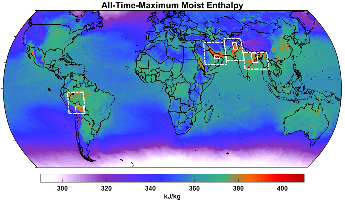 All-time maximum humid heat at each gridcell, as measured by moist enthalpy. Our initial ambition was a complete spatial (latitude+longitude+vertical) and temporal picture of heat and moisture states and fluxes in a variety of regions. Such a scope quickly proved impractical, so we settled on a more selective analysis of four regions (white boxes in figure above), which still encompass a diversity of meteorological and geographical factors. While the regions differ in many respects, two key characteristics ultimately emerged: places and times with globally extreme humid heat have abundant low-level moisture and no deep convection. Even slightly cooler sea-surface temperatures or slightly greater atmospheric instability were associated with substantially lower peak humid heat, which in previous work we've shown can occur for just a few hours before dropping to more manageable (but still oppressive) levels. We then leveraged these crude but robust correlations to predict locations of globally extreme humid heat using circulation, radiation, and flux proxies and cheating a bit by designing criteria to exclude certain climate regimes such as tropical rainforests. Nonetheless, our criteria include no information about the actual near-surface temperature or moisture patterns. Our predicted patterns match the observed ones fairly well (see figure below), particularly notable for the two regions with the highest humid heat -- South Asia and the Persian Gulf basin -- whose contrasting climates lead to quite different ways of achieving the high-moisture/no-convection combination. [This is explored in the paper.] The general idea of other regional maxima also agrees, such as northwest Mexico and northern coastal Australia. There are of course a number of places where the simple model gives under- or overestimates, including the western Amazon, central Africa, and northern Red Sea, and it generally underplays the risk of extreme humid heat over oceans. But the standards for success are always lower when there is a lack of direct precedent. 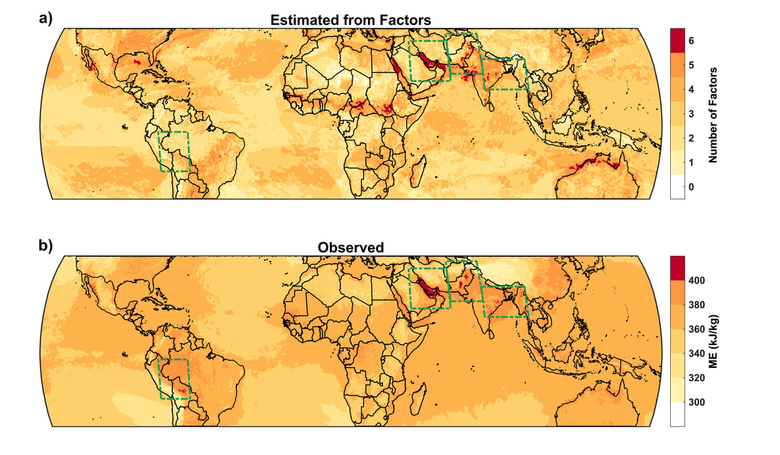 Empirical factors determining the geography of extreme humid heat. (a) Number of hypothesized important factors present at each grid cell, assessed via criteria involving nearby warm SSTs or large latent-heat fluxes; downward motion; exclusion of areas with extreme shortwave radiation; high but not extreme net longwave radiation; moderate annual-median relative humidity; and elevation <500 m. (b) Observed all-time humid-heat maximum (as measured by moist enthalpy). The complexity of Earth-system science, especially now that it is converging with other fields in recognition of our managed-planet reality, means that studies are often like forays into a cave with a lantern: they can raise an order of magnitude more questions than they answer. From our work, some of the most interesting would involve peeling back the onion skin another layer to discover, for example, precisely how topography aids in producing a stable shallow boundary layer in some regions and at some times (but not others), and the time-varying proportion of water vapor originating from marine versus continental sources (and its sensitivity to various atmospheric and marine perturbations). The former would help pinpoint climatological humid-heat hotspots, particularly in data-sparse areas with complex terrain; these hotspots are especially relevant as climate change lurches us closer to the 35C physiological survivability limit for sustained exposure. The latter would help determine how we might manage agriculture, urban, and energy systems to mitigate humid-heat extremes even incrementally, such as by limiting irrigation for critical several-day periods due to unfavorable synoptic conditions.
We hope the simplicity and generalized nature of our conclusions makes them useful as a basis for further work to closely examine processes in certain regions and at certain timescales; to consider the effects of mitigation or adaptation measures; or to understand time-dependent relationships with precipitation. Implementing a rigorous causal framework and using it as a constraint on data-driven machine learning would neatly expand on our work while retaining a level of parsimony and interpretability. Regrettably, humid heat will doubtless weigh more and more on people's minds, and their wallets, as climate change progresses. Marshalling a compendium of local and regional studies, that consider physical processes and their human-systems feedbacks across scales, is probably the single most effective tool for motivating meaningful individual and collective action; however, the flow of motivation can go both ways, as a coherent global framework can also prove invaluable for simplifying and linking research in ways that appeal to 'big-picture' thinking. Facing such a crucial and long-term global issue, all of these zoom levels must be pressed into service. Often discussed as an aspect of climate change is the idea that seasons will somehow be different than they have been in the recent past. How precisely they will differ, though, is exceptionally hard to pin down for analysis. For example, what defines 'spring'? Is it simply the transition between winter and summer? Is it a certain statistical distribution of temperature, precipitation, and cloudiness (not just their values but the combinations of them on certain days, the temporal sequences in which they occur, and so forth)? If May becomes substantially warmer, does that make it part of summer? How would we know?
It is these types of questions that have so far precluded meaningful seasonal-change analysis. One challenge is that seasons are so different from place to place -- both their first-order statistics, as noted, but also the experience of them. What would winter in New England be without abrupt cold fronts, or Great Plains summer with fewer thunderstorms? Such changes might not be readily apparent in temperature and precipitation averages, if compensated for example by increases in non-thunderstorm precipitation, but would lend the season a different feeling and influence impacts such as power outages. Similarly, particular combinations of weather patterns can be of immense cultural and/or agricultural significance. A moderate decrease in early-spring diurnal temperature variation may lead to a dramatically shorter maple-sugaring season in Vermont or Quebec, affecting sense of place. Crops that require chilling hours or moderate temperatures would necessarily see geographic shifts. Elsewhere, typical mid-latitude conceptions of distinct seasons do not apply, requiring a more careful multivariate depiction. Along the Southern California coast, for example, Santa Ana winds can cause the most intense heat of the year to occur in late autumn or even winter, leading to health impacts. This year, January, April, September, October, and November all saw higher temperatures in coastal Los Angeles than anything in June, July, or August. Extreme (or indeed unprecedented) events can color impressions and shape impacts of an entire season, despite relatively short durations. The incredible Pacific Northwest heatwave this summer stands as a canonical example. Even if the rest of the summer conformed closely to expectations, the die of memory (for humans, vegetation, soil, etc.) was already cast. That raises the question of the proper scope and timescale for attribution analyses, which are coming fast and furious these days. Event-based attribution to anthropogenic climate change is the standard, but by omitting the seasonal context, important information may be being lost. This is particularly important for multi-season events such as summer drought preconditioned by spring heat, fire-following mudslides, or spatially propagating droughts. One approach that holds promise for a more intuitive seasonal quantification involves a deeper investigation of 'weather types' -- in other words, reducing the dimensionality of weather by categorizing days into multivariate composite clusters. Changes in frequency of weather types could then indicate important shifts in seasonal behavior, perhaps concentrated at boundaries between seasons. But then here again several philosophical issues rear their head. First, whether to rely on actual values or values relative to an annual distribution -- warming, combined with a smaller winter/summer difference in a warmer world (continuing the pattern of greater winter warming that has occurred since the Last Glacial Maximum, also supported by longstanding model evidence), is the key underlying factor. Second, even an idealized conception of seasons has a 'ragged edge' where there is some alternation between weather typical of the preceding and the subsequent season. Evidently, each of the Köppen climate 'types' contain multitudes, some more important than others but all posing complications to assumptions about what meaningfully distinguishes one season or weather type from another. The most material impact of warming-driven seasonal change will involve behavioral practices that will have to shift along with changing environmental suitability due to physiological constraints (those of humans, animals, and/or crops). A rigid climatic shift where all patterns are identical except warmer by 2 or 3 deg C would mean that a once-pleasantly-warm summer outing becomes uncomfortable or dangerous, potentially leading to large-scale societal changes in the timing of activities (avoiding the warmest part of the day and/or the warmest time of the year). Of course, the thermodynamics of a warmer and moister atmosphere also drive exponentially intensifying extreme events, which often have contributions from changes in dynamics as well. Ultimately, the question of how to treat future seasons crystallizes a few of the principal issues in our collective understanding of a changing climate. Surely our ancestors of 15,000 years ago wrestled with some of the same problems, although with a different vocabulary and presumably less guilt, because there was little objective understanding of the situation (rapid glacial melting) and no perceived control over it. Despite (or even perhaps because of) reams of data, the world almost unavoidably requires narratives to imbue it with meaning. The concept of seasons is one such narrative. But they are a simplistic approximation of a complex system, and a threshold-based approach to a continuous problem. Both of these often lead to dramatic conclusions and misleading impressions. A relativistic definition of seasons across changing climates is without doubt the most basic approach, yet this conflicts with our closely held associations. Bringing our mindsets to a physical system is bound to get ourselves tied up in knots. As elegantly described in the essential climate-philosophy book "Climate Conundrums", Earth (and indeed life itself) has no values. *We* have values, but we shouldn't get confused into thinking these are objective or inevitable. Technology often outpaces principles, and following that idea, maybe it will turn out to be the case that changing the atmosphere, ocean, and land surface is the easy part, and adjusting our ideas and expectations to match the new reality that follows will prove significantly harder. Abstract Extreme events with decreasing trends in frequency or severity can still cause major disruptions to human or natural systems — as vividly illustrated by February’s winter storm in the south-central United States, which may ultimately become the costliest natural disaster in U.S. history. These impacts underscore that the path to comprehensive climate resilience runs through assessments of the structure and interconnections of systems, as well as narratives that emphasize the large variability around trends in extreme events. Main In mid-February 2021, widespread extreme cold paralyzed power and water systems in Texas and neighboring states (Figure 1). Seeing areas known for hurricanes and summer heat shivering amid near-record cold and snow was especially striking in light of observed trends and future projections emphasizing increases in heat, drought, flood, and fire.(1) The concept of ‘global weirding’ has gained prominence for describing this surficial paradox of increasing extremes in both tails of a distribution, a paradox which is readily resolved by recognizing several critical factors, including the ongoing amplification of certain hydrological processes and the (possibly temporary) destabilization of the boreal-winter polar vortex.(2,3) Here, I argue that weirding — the variability component of climate change — and its potential impacts be investigated more closely and systematically, using the Texas event as a lens into some of the key issues and categories of potential solution. Global-mean warming is causing the ‘leading edge’ of various hazards to shift, decade by decade, into locally unprecedented territory.(4) Appropriately, much effort and funding is being expended to assess the growing risks these hazards pose, and to determine optimal adaptation and mitigation strategies for them.(5) In fact, catastrophic risk theory argues that they perhaps merit even more attention, so as to fully understand low-probability, very-high-risk scenarios for the remainder of the 21st century and beyond.(6) In this context, the disaster in Texas serves as a reminder that extreme winter cold — and other ‘trailing-edge’ hazards such as cold wet springs (7) with observed or projected decreasing trends in frequency or severity — remain a critical source of risk, more than capable of overwhelming fragile societal systems. That this is possible, despite rapid warming, is due in part to a lack of generalized resilience in the affected systems and in part to anthropogenic networks which scramble, and in some cases amplify, the direct link between hazard and impact which would exist in a simpler world.(8) As illustration, extreme cold between February 10th and 17th spiked power demand across Texas to levels higher than the state’s electric grid could handle, and its isolation from interstate network connections, along with the inadequate winterization of natural-gas power plants and other critical infrastructure, led to multi-day power outages. Poorly insulated water pipes indoors and outdoors then froze and burst, causing serious damage to buildings and leaving millions of people without running water, exacerbating a humanitarian crisis. 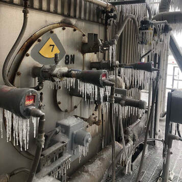 Figure 1: Icicles hang from frozen equipment at a natural-gas power plant in southeast Texas on February 15, 2021. Source: Entergy Texas (URL: https://www.entergynewsroom.com/article/entergy-texas-storm-update-2-15-21-5-p-m). The unfolding of this disaster points to two problems: a failure of knowledge (or awareness of that knowledge) and a failure of action. Much attention has focused on the latter issue, and justifiably, because recommendations following disruptive cold and snow events in Texas in 1989 and 2011 were mostly not followed through upon.(9) Designed to fit short-term climatologies and encompassing a spatial area too small to include meaningfully offsetting temperature anomalies, the state’s power grid has also seen strain from summer heat waves.(10) The issue of knowledge is somewhat more subtle but nonetheless crucial for optimal risk assessment and mitigation. Consider two episodes that affected Houston: the recent cold, and the flooding from 2017’s Hurricane Harvey. Both overwhelmed the city’s infrastructure, and both had impacts strongly shaped by investment, development, and policy decisions that often aggravated pre-existing socioeconomic inequalities.(11) However, although temperatures in Houston fall below -3C about annually, with -10C not uncommon across North Texas, freezing temperatures of sufficient duration and extent to cause serious impacts went unmentioned in a recent report on extreme-weather risks in the state (in contrast to tropical cyclones).(12) There are even indications that this ‘trailing-edge’ event could ultimately be the costliest natural disaster in US history, surpassing Harvey.(13) Beyond the recent headlines and regional anecdotes, the argument that a more complete picture of climate risk necessitates a deeper appreciation of trailing-edge-type events has several pillars. For one, there is evidence that the tails of the distribution of climate impacts are often thicker than models would suggest.(14) If true for the trailing edge as well as the leading edge, even large decreases in trailing-edge hazards might result in only small decreases in their impacts, for example due to downstream risk cascades.(15) At a more theoretical level, while the question of how much to value the future relative to the present (i.e., the economic discount rate) is a subjective one, this rate is nearly always negative — that is, avoiding harm now is worth the most. Skimming over events with decreasing trends in favor of preparation for the medium- and long-term future also requires a degree of presumption that societies are reasonably well-prepared for the set of extremes physically possible with (for example) 20th-century climate forcings. This may be true in isolated cases, but neglects the various resource impediments to optimal adaptation measures, as well as the crucial and dynamic role of societal modulation in shaping both events and their impacts.(16) The most direct way to ensure that trailing-edge risks are not underestimated lies in the framing of the narrative around extreme events, such as emphasizing how in many cases awareness and preparedness matter more than the magnitude of a hazard in determining its impacts. In both public-facing and intra-scientific discourse, this narrative could be furthered by portraying trailing-edge-type hazards over the next several decades as a threat that is very much present in most extratropical locations due to inherent climate-system variability. The emerging concept of multidimensional risk provides a helpful and widely applicable perspective, particularly relevant for its emphasis on the importance of specific combinations of extreme events rather than broad trends in any one variable. For example, the frequency of false springs (a period of warmth followed by a late frost) is expected to increase in some regions despite significant warming,(17) while rapid ‘whiplash’ between anomalous hydroclimatic states of opposite type is likely to accentuate both drought- and flood-related impacts in California.(18) Multi-hazard dependencies can also act to decrease risk compared with independent events.(19) Relative to a top-line emphasis on trends, this type of framing aids in placing into appropriate context the occurrence of any extreme events involving those variables, whether they are overall increasing or decreasing. A variety of complex relationships can be usefully explored through the framework of compound events (20), which considers the interaction of distinct variables or hazards as an integral driver of risk, and which can be extended to incorporate the substantial modulating effect of human systems like policies and transport networks.(8) Holistically evaluating climate risks also includes determining how much stands to be gained at the trailing edge in cases where risk is increasing at the leading edge. These benefits are often overshadowed, and rightly, by ramifications of the rapid and unrelenting increase in temperature to levels outside the range in which humans evolved.(21) But in a world where extreme cold still causes more mortality than extreme heat (22), the likely reduction of this harm by mean warming is worth exploring in greater detail. Similarly, that cities tend to be warmer than their surroundings is typically investigated as a summertime-heat problem, but it is equally valid to consider this urban-heat-island effect in moderating winter cold.(23) Many types of extreme events consistent with the current state of the climate system can lead to major harm when societies are not sufficiently resilient. In the recent Texas winter storm and cold spell, serious deficiencies in infrastructure were paired with critical socioeconomic vulnerabilities, as has been true for other recent disasters.(24) Although most focus deserves to remain on extreme events that are growing in prominence, due to their looming and poorly constrained impacts, trailing-edge-type risks cannot be neglected in refining scientific understanding or implementing resilience measures. Such a balance will help ensure that future climate extremes are not so disastrous, no matter what their location within statistical distributions or which combinations of systems they affect. References
1. Seneviratne, S. I., et al. (2012). A Special Report of Working Groups I and II of the Intergovernmental Panel on Climate Change (IPCC). Cambridge University Press. 2. Held, I. M., & Soden, B. J. (2006). J. Clim. doi:10.1175/jcli3990.1. 3. Cohen, J., et al. (2020). Nat. Clim. Change. doi:10.1038/s41558-019-0662-y. 4. Coumou, D., & Rahmstorf, S. (2012). Nat. Clim. Change. doi:10.1038/nclimate1452. 5. AghaKouchak, A., et al. (2020). Ann. Rev. Earth Planet. Sci. doi:10.1146/annurev-earth-071719-055228. 6. Lenton, T. M., et al. (2019). Nature. doi:10.1038/d41586-019-03595-0. 7. Faust, E., & Strobl, M. (2018). https://www.munichre.com/topics-online/en/ climate-change-and-natural-disasters/climate-change/ heatwaves-and-drought-in-europe.html 8. Raymond, C., et al. (2020). Nat. Clim. Change. doi:10.1038/s41558-020-0790-4. 9. Federal Energy Regulatory Commission and North American Electric Reliability Corporation. (2011). https://www.ferc.gov/sites/default/files/2020-04/08-16-11-report.pdf. 10. Krauss, C., Fernandez, M., Penn, I., & Rojas, R. (2021). New York Times. https://www.nytimes.com/2021/02/21/us/texas-electricity-ercot-blackouts.html. 11. Smiley, K. T. (2020). Environ. Res. Lett. doi:10.1088/1748-9326/aba0fe. 12. Nielsen-Gammon, J., Escobedo, J., Ott, C., Dedrick, J., & Van Fleet, A. (2020). https://climatexas.tamu.edu/products/texas-extreme-weather-report/ClimateReport-NOV2036-2.pdf. 13. Ivanova, I. (2021). CBS News. https://www.cbsnews.com/news/texas-winter-storm-uri-costs. 14. Schewe, J., et al. (2019). Nat. Commun. doi:10.1038/s41467-019-08745-6. 15. De Ruiter, M. C., et al. (2020). Earth’s Future. doi:10.1029/2019ef001425. 16. United Nations Office for Disaster Risk Reduction (2019). eISBN: 978-92-1-004180-5. 17. Allstadt, A. J., et al. (2015). Environ. Res. Lett. doi:10.1088/1748-9326/10/10/104008. 18. Swain, D. L., Langenbrunner, B., Neelin, J. D., & Hall, A. (2018). Nat. Clim. Change. doi:10.1038/s41558-018-0140-y. 19. Hillier, J. K., & Dixon, R. S. (2020). Environ. Res. Lett. doi:10.1088/1748-9326/abbc3d. 20. Zscheischler, J., et al. (2020). Nat. Rev. Earth Environ. doi:10.1038/s43017-020-0060-z. 21. Xu, C., Kohler, T. A., Lenton, T. M., Svenning, J.-C., & Scheffer, M. (2020). Proc. Nat. Acad. Sci. doi:10.1073/pnas.1910114117. 22. Gasparrini, A., et al. (2015). Lancet. doi:10.1016/S0140-6736(14)62114-0. 23. Yang, J., & Bou-Zeid, E. (2018). J. Appl. Meteorol. Climatol. doi:10.1175/jamc-d-17-0265.1. 24. Kishore, N., et al. (2018). N. Engl. J. Med. doi:10.1056/nejmsa1803972. |
Archives
September 2023
Categories |
 RSS Feed